An Introduction to R Language
啟動 R 後, 可以看到下面的視窗環境:
c (x, y, z, ...)
c (1,7:9)
c (1:5, 10.5, "next")
向量的運算:
t (x) – transpose of x 轉置
讀取 Excel 的 CSV 檔案 read.csv :
如果檔案 mlb.csv 內容是
Teams,W,ERA,R,OBP,SLG,AVG
Baltimore Orioles,66,4.59,613,0.316,0.386,0.259
Boston Red Sox,89,4.2,818,0.339,0.451,0.268
……
Toronto Blue Jays,85,4.22,755,0.312,0.454,0.248
讀入資料的指令並存成一個 data frame是:
> team_stats = read.csv ("d:\\hcwang\\R\\mlb.csv", head=TRUE, sep=",")
顯示data frame變數 team_stats的內容 (data frame 是 R 語言的一種資料型態)
> team_stats
Teams W ERA R OBP SLG AVG
1 Baltimore Orioles 66 4.59 613 0.316 0.386 0.259
2 Boston Red Sox 89 4.20 818 0.339 0.451 0.268
……
14 Toronto Blue Jays 85 4.22 755 0.312 0.454 0.248
> names ( team_stats )
[1] "Teams" "W" "ERA" "R" "OBP" "SLG" "AVG"
取得其中一個欄位(如ERA)的資料:
> team_stats$ERA
[1] 4.59 4.20 4.09 4.30 4.30 4.97 4.04 3.95 4.06 3.56 3.93 3.78 3.93 4.22
可以使用 attributes 得知data frame變數 team_stats的內容敘述
> attributes (team_stats)
$names
[1] "Teams" "W" "ERA" "R" "OBP" "SLG" "AVG"
$class
[1] "data.frame"
$row.names
[1] 1 2 3 4 5 6 7 8 9 10 11 12 13 14
write (x, file = "filename", ncolumns = m, append = FALSE, sep = " ")
x - the
data to be written out. If
x is a
two-dimensional matrix you need to transpose it to
get the columns in
file
the same as those in the internal representation.
sep - a string used
to separate columns. Using
sep = "\t"
gives tab delimited output;
default is
" "
Example:
> write ("\n This is a test. \n\n", file="output.prn") - \n 是跳到新的一列
> x = matrix (1:10, ncol = 5)
> x
[,1] [,2] [,3] [,4] [,5]
[1,] 1 3 5 7 9
[2,] 2 4 6 8 10
使用 append=TRUE, 可寫入後續的資料.
> write ( t (x), file="output.prn", ncolumns=5, sep=" ", append=TRUE)
備註: 如果沒使用 t (x),
> write ( x, file="output.prn", ncolumns=5, sep=" ", append=TRUE)
則會輸出
1 2 3 4 5
6 7 8 9 10
將執行的結果寫入檔案的指令:
sink (file = NULL, append = FALSE, type = c("output", "message"), split=FALSE)
Example:
> sink(file = "sink2.txt",type = c("output", "message"), split=TRUE)
> i=1:5
> i
> sink() ## 結束
如果要刪除該檔案, 可用 unlink 指令
> unlink("sink2.txt")
Probability 指令:
|
Distribution |
Normal |
t- |
Binomial |
|
|
Probability density function 機率密度函數 |
dnorm |
dt |
dbinom |
dchisq |
|
Cumulative probability density function |
pnorm |
pt |
pbinom |
pchisq |
|
Inverse cumulative probability density function |
qnorm |
qt |
qbinom |
qchisq |
|
Random numbers |
rnorm |
rt |
rbinom |
Rchisq |
Example:
> dnorm (-5:5, mean = 0, sd = 1 )
[1] 1.486720e-06 1.338302e-04 4.431848e-03 5.399097e-02 2.419707e-01 3.989423e-01
[7] 2.419707e-01 5.399097e-02 4.431848e-03 1.338302e-04 1.486720e-06
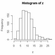
畫圖指令
Example:
> z = rchisq (1000, df = 10)
> hist (z)
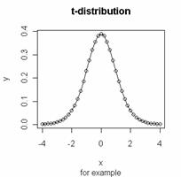
> x = seq (-4, 4, by = 0.2 )
> y = dt (x, df = 10 )
> plot (x, y, type = "o")
> title ( main = "t-distribution", sub = "for example" )
type = "p" – points only
"l" – line only
"b" – both
"o" – for both over-plotted
> x=1:10

> boxplot (x, main="Test")
計算信賴區間 Confidence Interval From a Normal Distribution
> x = 5
> sigma = 2
> n = 20
> error = qnorm(0.975) * sigma / sqrt(n) ## 1-0.05/2 = 0.975
> left = x - error
> right = x + error
> left
[1] 4.123477
> right
[1] 5.876523
P 值的計算
> xbar = 7
> z = ( x – xbar )/ ( sigma / sqrt(n))
> z
[1] -4.472136
> 2 * pnorm (-abs(z)) ## Large samples
[1] 7.744216e-06
> 2 * pt(-abs(z),df = n-1) ## Small samples
[1] 0.0002611934
因為
p 值小於
0.05, 所以拒絕虛無假設
![]() .
.
控制敘述指令:
Conditionals Execution
if ( condition_expression )
{ if_expression_1;
if_expression_2;
…
}
else
{ else_expression_1;
…
}
迴圈控制
for (var in seq)
{
expression_1;
expression_2;
…
}
Example:
> s = 0
> for (i in 1:length (x)) {
+ s = s + x[i]
+ }
> s
[1] 55
while (condition) { expr … }
可以使用 break 離開(跳出)迴圈. 而使用 next, 則可以進行迴圈的下一個計算
ifelse – 邏輯運算
Example:
> x = 1:5
> x > 3
[1] FALSE FALSE FALSE TRUE TRUE
> ifelse ( x > 3, 1, 0 )
[1] 0 0 0 1 1
函式 (函數) 敘述
name = function(arg_1, arg_2, ...) {
expression 1
expression 2
……
}
Examples:
> hello = function(x,y) { x^2+y^2 }
> hello(2,3)
[1] 13
> hello ( 1:3, 3:5)
[1] 10 20 34